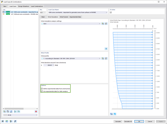
If you have experimentally determined surface pressures available for a model, you can apply them to a structural model in RFEM 6, process them in RWIND 2, and use them as wind loads in the structural analysis of RFEM 6.
You can find out how to apply the experimentally determined values in this technical article.

The modal relevance factor (MRF) can help you to assess to which extent specific elements participate in a specific mode shape. The calculation is based on the relative elastic deformation energy of each individual member.
The MRF can be used to distinguish between local and global mode shapes. If multiple individual members show significant MRF (for example, > 20%), the instability of the entire structure or a substructure is very likely. On the other hand, if the sum of all MRFs for an eigenmode is around 100%, a local stability phenomenon (for example, buckling of a single bar) can be expected.
Furthermore, the MRF can be used to determine critical loads and equivalent buckling lengths of certain members (for example, for stability design). Mode shapes for which a specific member has small MRF values (for example, < 20%) can be neglected in this context.
The MRF is displayed by mode shape in the result table under Stability Analysis → Results by Members → Effective Lengths and Critical Loads.
- Analysis of time diagrams and accelerograms (acceleration-time diagrams exciting the supports of a structure)
- Combination of user-defined time diagrams with nodal, member, and surface loads, as well as free and generated loads
- Combination of several independent excitation functions
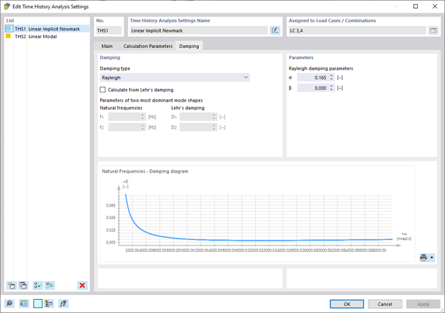
- Linear implicit Newmark analysis or modal analysis in time history
- Structural damping using Raleigh damping coefficients or Lehr's damping value
- Graphical display of results in calculation diagrams
- Result display in individual time steps or as an envelope during the entire time period
- Extensive library of seismic events (accelerograms)
The model and loads are entered as usual in the RFEM interface.
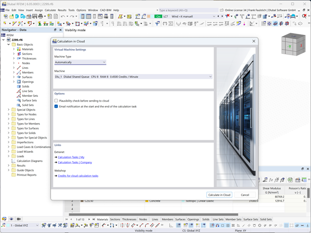
You can start the cloud calculation by selecting an entry in the Calculate menu. Then, select the virtual machine suitable for the task and start the calculation.
After the start, the image is used to create a virtual machine on which the computing server is started. This takes over the calculation of your file.
You can monitor the processing of calculation tasks in the Extranet.
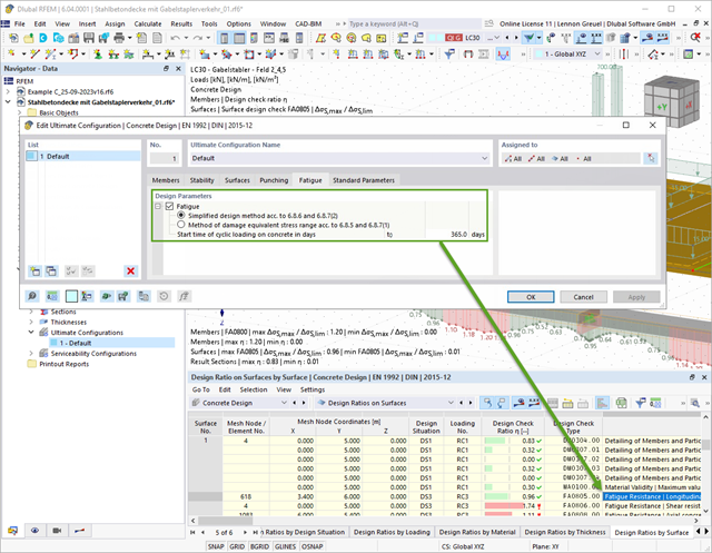
With the Concrete Design add-on, you can perform the fatigue design of members and surfaces according to EN 1992‑1‑1, Chapter 6.8.
For the fatigue design, you can optionally select two methods or design levels in the design configurations:
- Design Level 1: Simplified design according to 6.8.6 and 6.8.7(2): The simplified design is performed for frequent action combinations according to EN 1992‑1‑1, Chapter 6.8.6 (2), and EN 1990, Eq. (6.15b) with the traffic loads relevant in the serviceability state. A maximum stress range according to 6.8.6 is designed for the reinforcing steel. The concrete compressive stress is determined by means of the upper and lower allowable stress according to 6.8.7(2).
- Design Level 2: Design of damage equivalent stress acc. to 6.8.5 and 6.8.7(1) (simplified fatigue design): The design using damage equivalent stress ranges is performed for the fatigue combination according to EN 1992‑1‑1, Chapter 6.8.3, Eq. (6.69) with the specifically defined cyclic action Qfat.
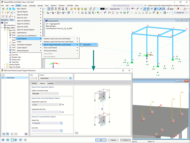
Use the "Import Support Reactions" Load Wizard in RFEM 6 and RSTAB 9 to easily transfer reaction forces from other models. The wizard allows you to connect all or several nodal and line loads of different models with each other in a few steps.
The load transfer from load cases and load combinations can be carried out automatically or manually. It's necessary that the models are saved in the same Dlubal Center project.
The "Import Support Reactions" load wizard supports the concept of positional statics and allows you to digitally connect the individual positions.
Go to Explanatory Video
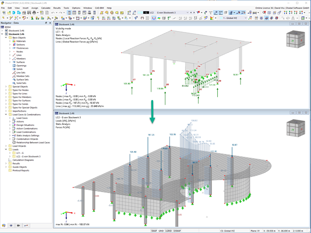
Using the "Load Transfer Only" story type, you can consider slabs without stiffness effect in and out of the plane in the Building Model add-on. This element type collects the loads on the slab and transfers them to the supporting elements of a 3D model. Thus, you can simulate secondary components, such as grillage and similar load distribution elements, without any further effect in the 3D model.
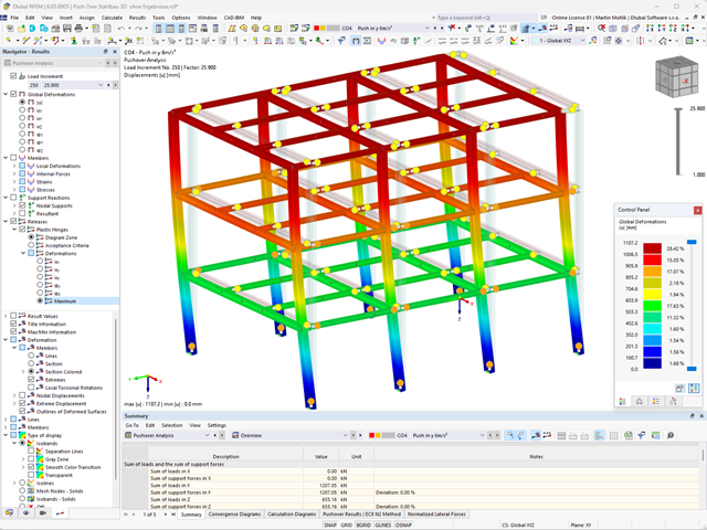
- Consideration of nonlinear component behavior using plastic standard hinges for steel (FEMA 356, EN 1998‑3) and nonlinear material behavior (masonry, steel - bilinear, user-defined working curves)
- Direct import of masses from load cases or combinations for the application of constant vertical loads
- User-defined specifications for the consideration of horizontal loads (standardized to a mode shape or uniformly distributed over the height of the masses)
- Determination of a pushover curve with selectable limit criterion of the calculation (a collapse or limit deformation)
- Transformation of the pushover curve into the capacity spectrum (ADRS format, single degree of freedom system)
- Bilinearization of the capacity spectrum according to EN 1998‑1:2010 + A1:2013
- Transformation of the applied response spectrum into the required spectrum (ADRS format)
- Determination of target displacement according to EC 8 (the N2 method according to Fajfar 2000)
- Graphical comparison of the capacity and required spectrum
- Graphical evaluation of the acceptance criteria of predefined plastic hinges
- Result display of the values used in the iterative calculation of the target displacement
- Access to all results of the structural analysis in the individual load levels
This function provides you with the option to adopt reaction forces from other models as nodal and line loads.
The option not only transfers the reaction load as an action, but digitally couples the support load of the original model with the load size of the target object. The subsequent changes in the original model are automatically adopted in the target model.
This technology supports the concept of positional statics and allows you to digitally connect the individual positions of the same Dlubal Center project.
Go to Explanatory Video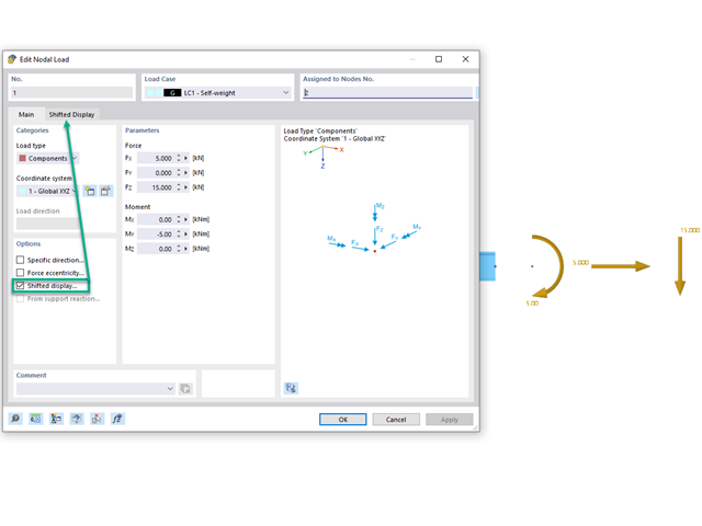
Would you like to display nodal loads or load components that act on one point next to each other? Then use the "Shifted Display" option. This allows you to define offsets in the x, y, and z directions, as well as the size and spacing.
Go to Explanatory Video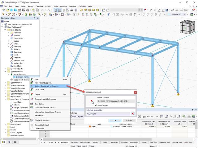
The object types listed below can be graphically assigned to the elements of the structure modeled in the program.
- Nodal supports
- Member shear panels
- Local reductions of member cross-sections
- Member transverse stiffeners
- Member longitudinal welds
- Effective lengths
- Boundary conditions
- Line supports
- Loads
- Member support
- Punching reinforcements
- Mesh refinements
- Surface reinforcements
- Surface results adjustments
- Surface support
- Service classes
- Imperfections

Do you want to consider other loads as masses in addition to the static loads? The program allows that for nodal, member, line and surface loads. For this, you need to select the Mass load type when defining the load of interest. Define a mass or mass components in the X, Y, and Z directions for such loads. For nodal masses, you have an additional option to also specify moments of inertia X, Y, and Z in order to model more complex mass points.

You can already see it in the image: Imperfections can also be taken into account when defining a modal analysis load case. The imperfection types that you can use in the modal analysis are notional loads from load case, initial sway via table, static deformation, buckling mode, dynamic mode shape, and group of imperfection cases.

You have several options available to define masses for a modal analysis. While the masses due to self-weight are considered automatically, you can consider the loads and masses directly in a load case of the modal analysis type. Do you need more options? Select whether to consider full loads as masses, load components in the global Z-direction, or only the load components in the direction of gravity.
The program offers you an additional or alternative option for importing masses: A manual definition of load combinations as of which are the masses considered in the modal analysis. Have you selected a design standard? You can then create a design situation with the Seismic Mass combination type. Thus, the program automatically calculates a mass situation for the modal analysis according to the preferred design standard. In other words: The program creates a load combination on the basis of the preset combination coefficients for the selected standard. This contains the masses used for the modal analysis.
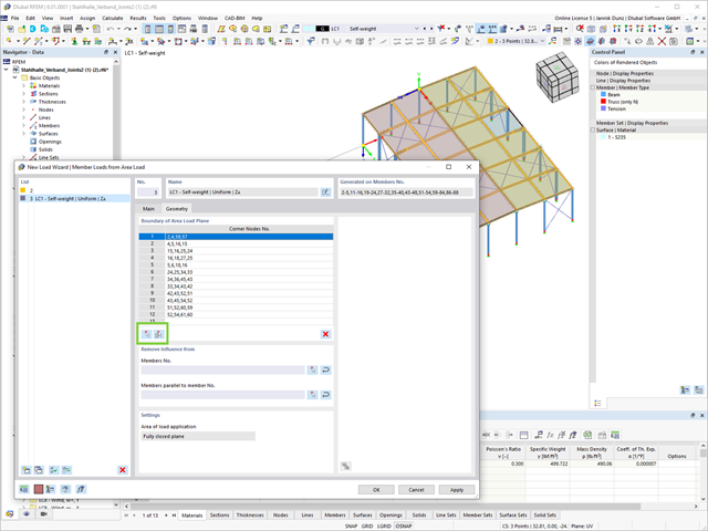
Another useful features in the Load Wiyard is the determination of member loads from area loads by defining surfaces (using corner nodes) and cells in a definition.
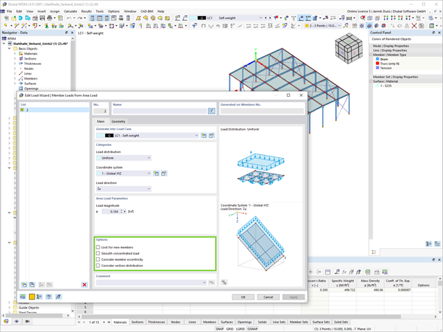
To make your work effiecient and quick, we have added new features to the load wizard. These include locking new members, smoothing occurring concentrated loads, and considering eccentricities as well as cross-section distribution.
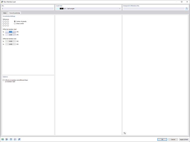
Always keep an eye on the stability of your structures: You can now consider eccentricities for nodal and member loads.
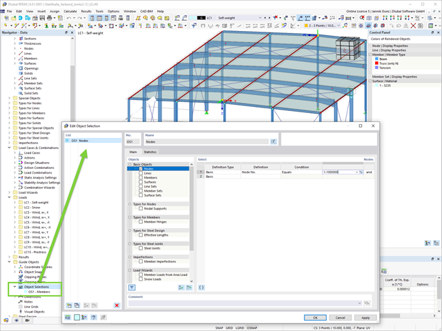
This feature creates more order. The new guide object "Object Selection" allows for generic filtering of various objects:
- Basic Objects
- Types for Nodes
- Types for Lines
- Types for Surfaces
- Load Wizards
- Loads
- Guide Objects
The object selection provides you with many interactive application possibilities at various program locations.
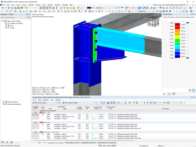
Do you work with steel connections? The Steel Joints add-on for RFEM supports you when analyzing steel connections by using an FE model. In this case, the modeling runs fully automatically in the background. Nevertheless, you can control this process via the simple and familiar input of components. You can then use the loads determined on the FE model for your design of the components according to EN 1993‑1‑8 (including National Annexes).
More About Steel Joints
- Calculation of stationary incompressible turbulent wind flow using the SimpleFOAM solver from the OpenFOAM® software package
- Numerical scheme according to the first and second order
- Turbulence models RAS k-ω and RAS k-ε
- Consideration of surface roughness depending on model zones
- Model design via VTP, STL, OBJ, and IFC files
- Operation via bidirectional interface of RFEM or RSTAB for importing model geometries with standard-based wind loads and exporting wind load cases with probe-based printout report tables
- Intuitive model changes via drag & drop and graphical adjustment assistance
- Generation of a shrink-wrap mesh envelope around the model geometry
- Consideration of environmental objects (buildings, terrain, and so on)
- Height-dependent description of the wind load (wind speed and turbulence intensity)
- Automatic meshing depending on a selected depth of detail
- Consideration of layer meshes near the model surfaces
- Parallelized calculation with optimal utilization of all processor cores of a computer
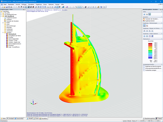
- Graphical output of the surface results on the model surfaces (surface pressure, Cp coefficients)
- Graphical output of the flow field and vector results (pressure field, velocity field, turbulence – k-ω field, and turbulence – k-ε field, velocity vectors) on Clipper/Slicer planes
- Display of 3D wind flow via animated streamline graphics
- Definition of point and line probes
- Multilingual user interface (German, English, Czech, Spanish, French, Italian, Polish, Portuguese, Russian, and Chinese)
- Calculations of several models in one batch process
- Generator for creating rotated models to simulate different wind directions
- Optional interruption and continuation of the calculation
- Individual color panel per result graphic
- Display of diagrams with separate output of results on both sides of a surface
- Output of the dimensionless wall distance y+ in the mesh inspector details for the simplified model mesh
- Determination of the shear stress on the model surface from the flow around the model
- Calculation with an alternative convergence criterion (you can select between the residual types pressure or flow resistance in the simulation parameters)
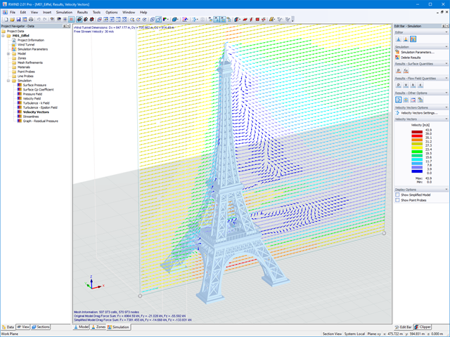
RWIND Basic uses a numerical CFD model (Computational Fluid Dynamics) to simulate wind flows around your objects using a digital wind tunnel. The simulation process determines specific wind loads acting on your model surfaces from the flow result around the model.
A 3D volume mesh is responsible for the simulation itself. For this, RWIND Basic performs an automatic meshing on the basis of freely definable control parameters. For the calculation of wind flows, RWIND Basic provides you with a stationary solve and RWIND Pro provides a transient solver for incompressible turbulent flows. Surface pressures resulting from the flow results are extrapolated onto the model for each time step.
When starting the analysis in the RFEM or RSTAB application, you trigger a batch process. It places all member, surface, and solid definitions of the model rotated with all relevant coefficients in the numerical wind tunnel of RWIND Basic. Furthermore, it starts the CFD analysis, and returns the resulting surface pressures for a selected time step as FE mesh nodal loads or member loads into the respective load cases of RFEM or RSTAB.
These load cases which contain RWIND Basic loads can then be calculated. Moreover, you can combine them with other loads in load and result combinations.
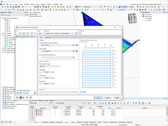
Discover the new features in RFEM and RSTAB for the determination of wind loads using RWIND:
- Useful load wizards for generating wind load cases with different flow fields in different wind directions
- Wind load cases with freely assignable analysis settings including a user-defined specification of the wind tunnel size and wind profile
- Comprehensive display of the wind tunnel with input wind profile and turbulence intensity profile
- Visualization and use of the RWIND simulation results
- Global definition of a terrain (horizontal planes, inclined plane, table)
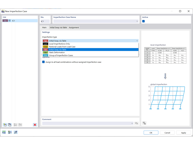
The organization of imperfections is efficiently solved by imperfection cases. The cases allow you to describe an imperfection from local imperfections, equivalent loads, initial sway via table (new), a static deformation, a buckling mode, a dynamic mode shape, or a combination of all these types (new).
Go to Explanatory Video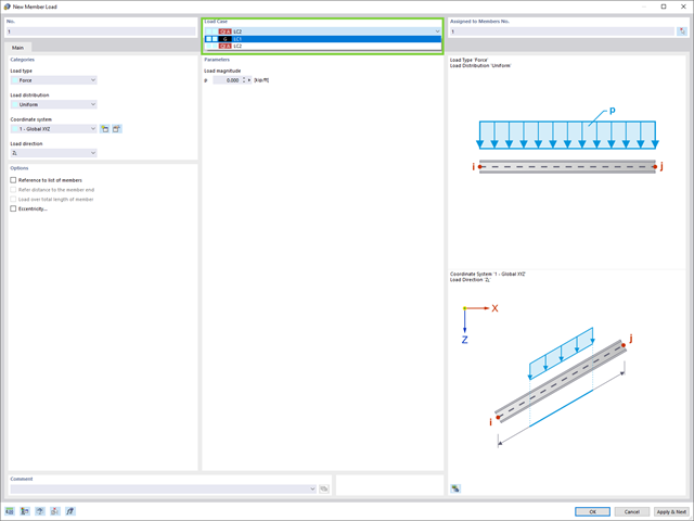
This feature is useful for your daily work! For member loads, surface loads, and so on, you can retroactively move loads into another load case.
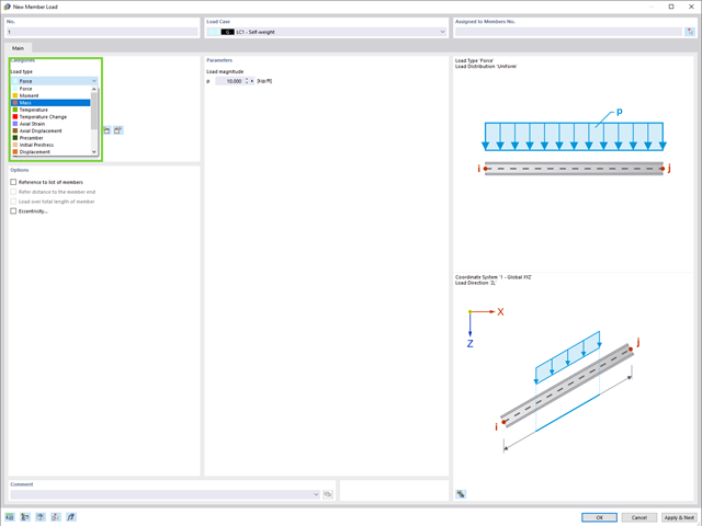
There is also an innovation in the load catalog that will interest you: The Mass Loads type has been added to the catalog!
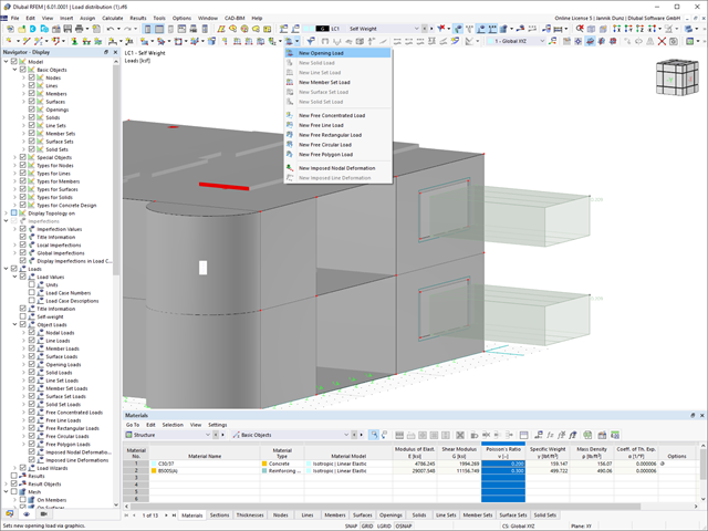
This new feature allows you to easily define opening loads (for example, wind loads) for flat loads on openings.
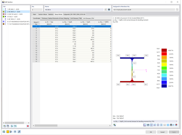
Make sure nothing collapses on you: To estimate the resistance of member cross-sections, it is possible to display the unit stresses for the unit loads N = 1 kiP, My = 1 kiP/ft, and so on, when selecting the cross-sections.
Go to Explanatory Video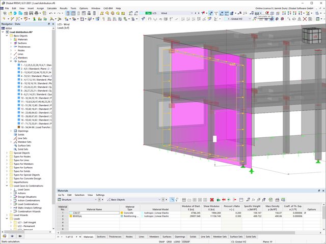
Keep an eye on all surfaces. A surface with the "Load Transfer" stiffness type has no structural effect. You can use it to consider the loads from surfaces that have not been modeled, for example, facade structures, glass surfaces, trapezoidal roof sections, and so on.
Go to Explanatory Video
Compared to the RF-/STEEL Warping Torsion add-on module (RFEM 5 / RSTAB 8), the following new features have been added to the Torsional Warping (7 DOF) add-on for RFEM 6 / RSTAB 9:
- Complete integration into the environment of RFEM 6 and RSTAB 9
- 7th degree of freedom is directly taken into account in the calculation of members in RFEM/RSTAB on the entire system
- No more need to define support conditions or spring stiffnesses for calculation on the simplified equivalent system
- Combination with other add-ons is possible, for example for the calculation of critical loads for torsional buckling and lateral-torsional buckling with stability analysis
- No restriction to thin-walled steel sections (it is also possible to calculate ideal overturning moments for beams with massive timber sections, for example)